网络营销措施有哪些武汉整站seo数据上云
文章目录
- 常见的CNN
- Alexnet
- 1乘1的卷积
- VGG网络
- Googlenet(Inception V1、V2、V3)
- 全局平均池化
- 总结
- Resnet、Resnext
- ResNet残差网络
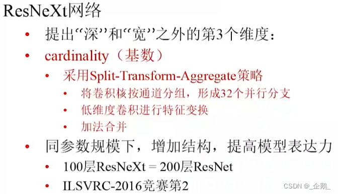
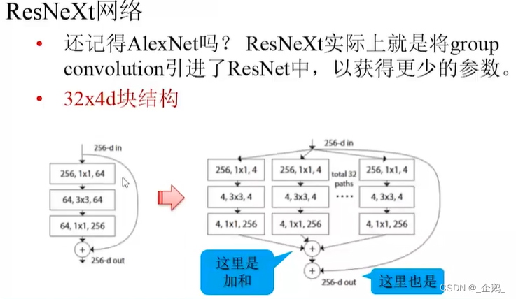
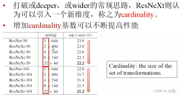
- ResNeXt网络
- 应用案例
- VGG
- Resnet
常见的CNN
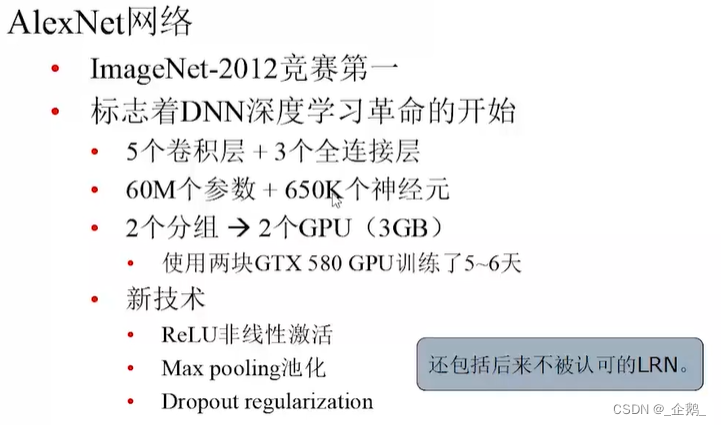
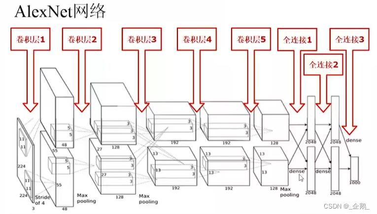
Alexnet
DNN深度学习革命的开始
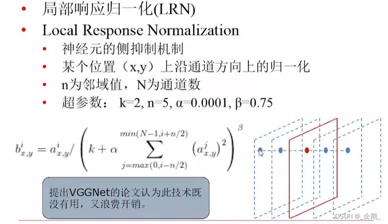
沿着窗口进行归一化。
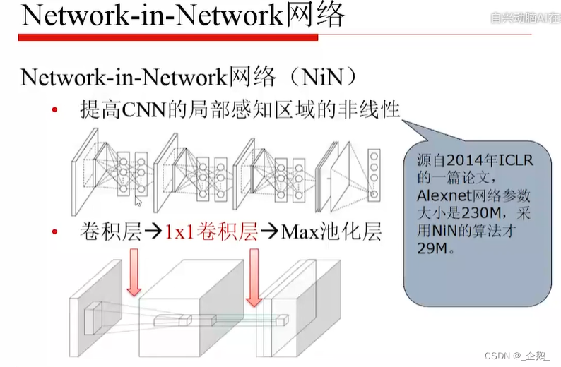
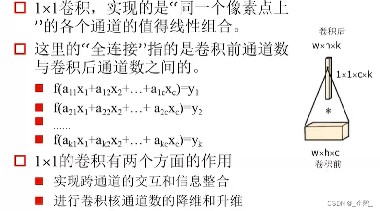
1乘1的卷积
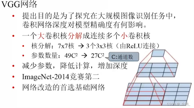
VGG网络
层数变多了。
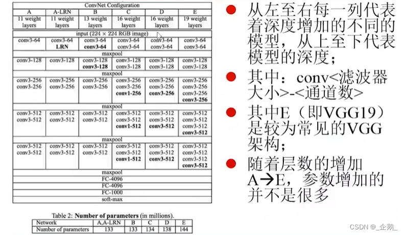
五层→五组
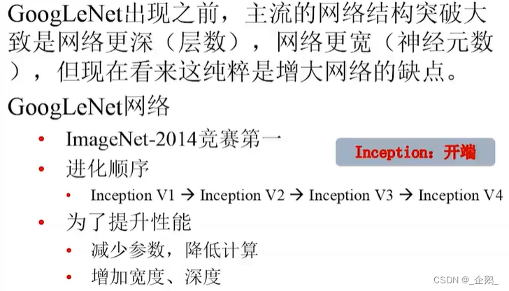
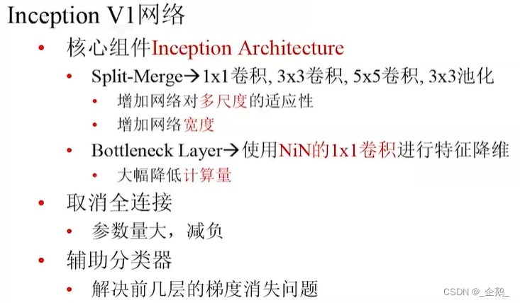
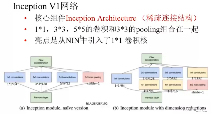
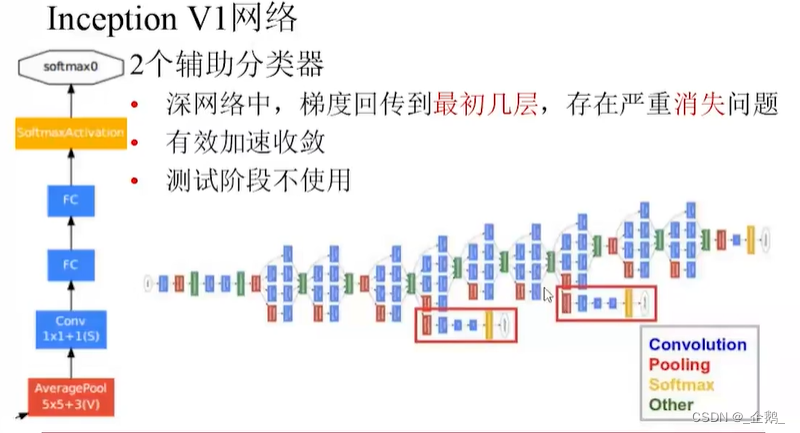
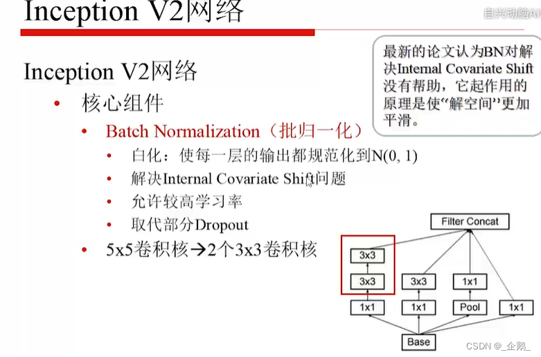
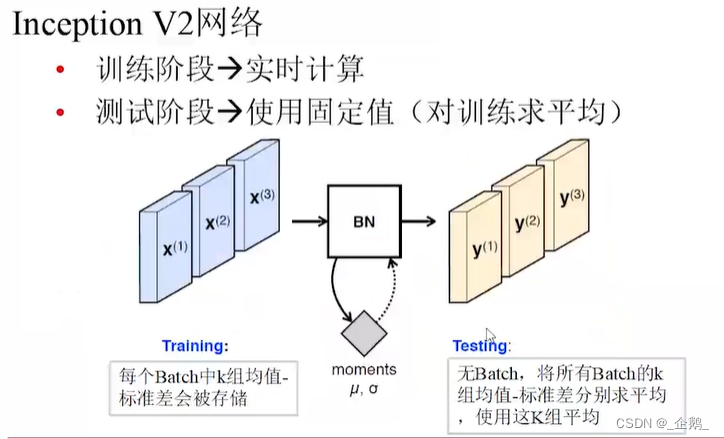
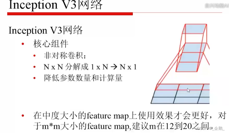
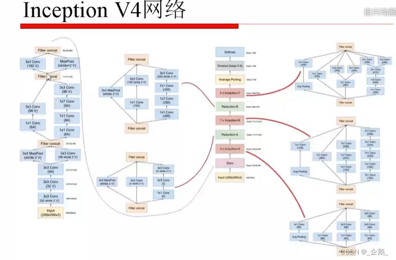
Googlenet(Inception V1、V2、V3)
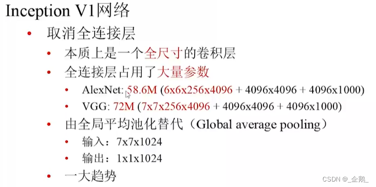
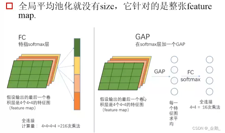
全局平均池化
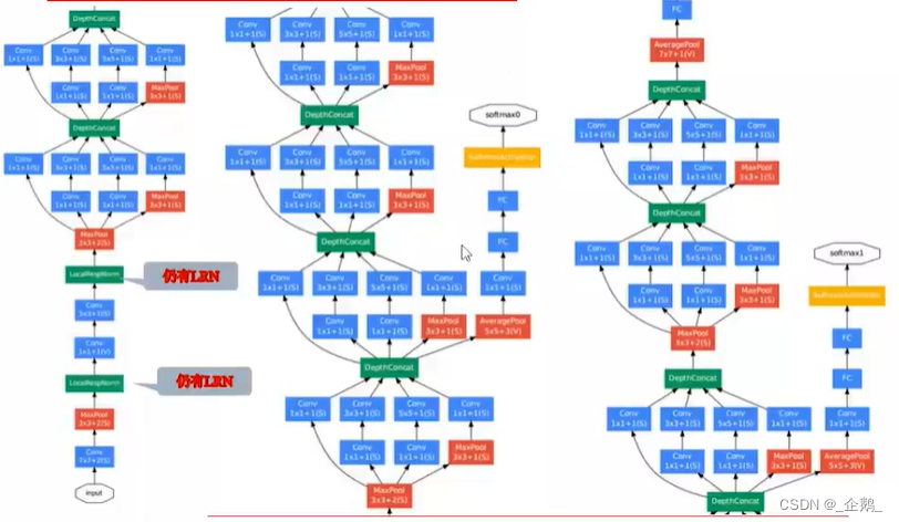
- 不增加计算量
- 避免表达瓶颈
- 增强结构(表达力),如宽度、深度。
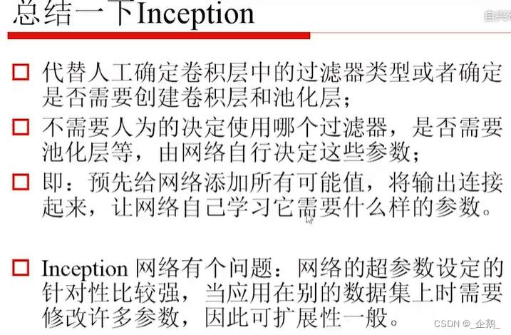
总结
Resnet、Resnext
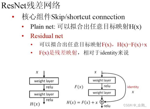
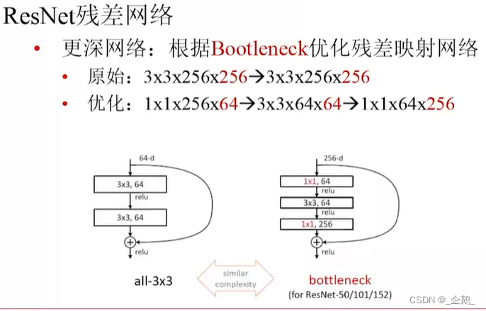
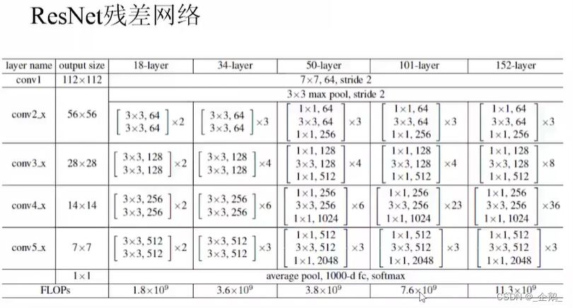
ResNet残差网络
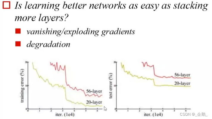
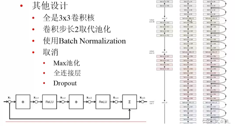
没有池化过程
变得很深
先降维再升维
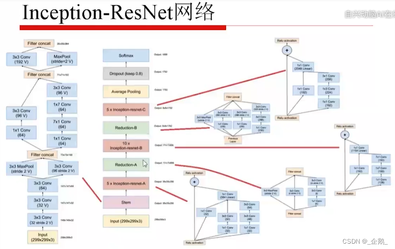
亮点在采用了残差的机制。
ResNeXt网络