后台java语言做网站软文素材网
在.NET 2025.1版本中,我们带来了巨大的期待功能,进一步简化了报告模板的开发过程。新功能包括通过添加链接报告页面、异步报告准备、HTML段落旋转、代码文本编辑器中的文本搜索、WebReport图像导出等,大幅提升用户体验。
FastReport .NET 是适用于.NET Core 3,ASP.NET,MVC和Windows窗体的全功能报告库。使用FastReport .NET,您可以创建独立于应用程序的.NET报告。
添加带有链接的报告页面
在以前的版本中,可以将另一份报告的页面添加到一份报告中。此选项可在 “文件->打开页面...”中找到。 默认情况下,页面的副本会添加到报告中。
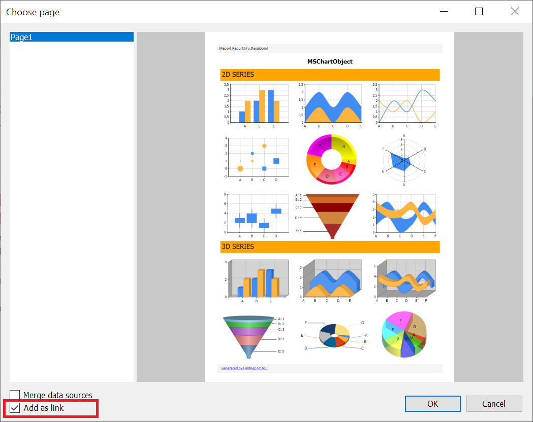
您现在可以启用“添加为链接”选项,该选项会将页面的链接添加到报告,而不是页面的副本。这意味着当您更改原始报告中的页面时,更改将反映在以链接形式添加该页面的所有报告中。反之亦然,如果在具有指向该页面的链接的报告中更改了页面,则原始报告中也会更改该页面。
异步报告准备
添加了report.PrepareAsync()方法,除了现有的同步report.Prepare()方法外,还支持异步报告准备。此方法还支持CancellationToken,允许用户在需要时取消报告准备过程,从而改善非阻塞环境中大型报告的控制和性能。此功能将来可能会进一步增强,新方法可提供额外的异步访问。
IfNull 函数
object IfNull(object expression, object defaultValue)
有一个新的函数允许 System.NullReferenceException在评估表达式时避免这种情况。该函数有两个参数:第一个是要评估的表达式,第二个是默认值。如果表达式可以评估,则函数返回其结果。如果不能,则返回默认值。
使用 TextRenderType.HtmlParagraph 旋转文本
添加了使用 TextRenderType.HtmlParagraph 旋转文本的支持。以前,文本旋转仅适用于其他文本渲染器类型。您可以在下面看到文本旋转的示例。
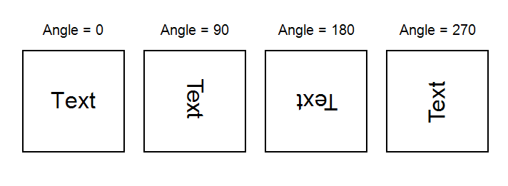
此外,现在可以正确将此类文本导出为 PDF。
FastReport WPF 和 FastReport Mono 代码编辑器中的文本搜索
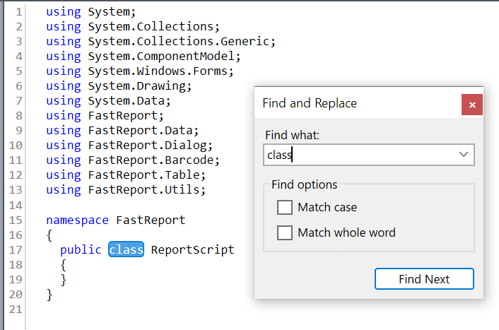
现在您不仅可以在 FastReport .NET 代码编辑器中搜索文本,还可以在 FastReport WPF 和 FastReport Mono 编辑器中搜索文本。
在FastReport WPF代码中搜索文本的示例:
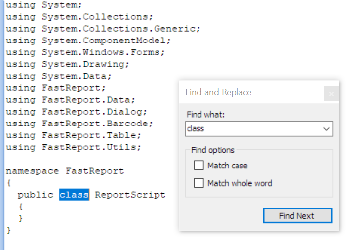
在 FastReport Mono 代码编辑器中:
Blazor WASM WebReport 的本地化支持
在 FastReport Blazor WebAssembly 中引入了对 WebReport 接口的本地化支持。以前,本地化是通过基于文件的方法进行管理的,这与 WASM 环境不兼容。新方法webReport.SetLocalization(Stream)允许从 Stream 加载本地化,使其与 Blazor WASM 应用程序兼容。
图像导出至WebReport
添加了将报告导出到图像的功能。要将其显示在导出列表中,请添加以下代码:
WebReport.Toolbar.Exports.ShowImageExport = true;
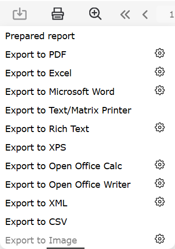
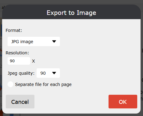
添加了将报告导出到图像的功能。要将其显示在导出列表中如果需要,您必须启用 WebReport 选项来配置导出到图像 WebReport.Toolbar.Exports.EnableSettings。启用后,您可以单击“齿轮”并在出现的模式窗口中更改设置。,请添加以下代码:
WebReport.Toolbar.Exports.ShowImageExport = true;
完整变更列表
[Engine]
+ 为 RichObject 添加了 PicturesInParagraph 属性;
+ 添加了异步报告准备方法 PrepareAsync();
+ 添加了将字符串转换为兼容 dbtype 的功能;
+ 添加了打印比例;
+ 在 ToWords 函数中添加了将单词转换为十进制的功能;
+ 添加了西班牙语的区域标识符 22538(西班牙语 - 拉丁美洲)和 3082(西班牙语 - 西班牙(现代排序));
+ 添加了新的 IfNull 函数用于处理表达式。如果表达式不为空,则返回计算表达式的结果,否则返回指定的默认值;
+ 实现了 RichObject 中图片水平位置的计算;
+ 添加了以虚拟主机样式发送请求的功能;
+ 添加了对 TextRenderType = HtmlParagraph 的文本旋转的支持;
+ 添加了为 Totals 的“PrintOn”属性使用标题带的功能;
* 升级了 FastReport.Data.OracleODPCore 中的 Oracle.ManagedDataAccess.Core;
* 将 GetConnection、OpenConnection 和 Dispose 方法标记为虚拟;
* 为 Hyperlink.Value 属性的传入值添加了空值检查;
* 静态验证方法 TryParse 已被引入到 QRCodes 类中;
- 修复了文本中断问题;
- 修复了 PageStart 事件后页面可见性变化的问题;
- 修复了转换为参数类型的问题;
- 修复了检查报告脚本中是否包含停用词(如果变量名称中包含停用词)的问题;
- 修复了启用 GrowToBottom 时文本对象底部边框的可见性问题;
- 修复了分组 DataBand 具有 GrowToBottom 选项时边框加倍的问题;
- 删除了 SVGPictureObject 中子 clipPath 标签的渲染;
- 修复了 FinishReport 事件中的一个错误;
- 删除了将 SubreportObject 添加到 ContainerObject 的无效功能;
- 修复了更改请求的 CommandType(如果已在 GetAdapter 中设置)的问题;
[设计器]
+ 添加了从另一个报告以链接形式打开页面的功能;
+ 为 span 标签添加了斜体、粗体、下划线和删除线字体样式;
+ 添加了通过键盘输入的字符在 TreeView 中进行搜索的功能;
+ 在 WPF 和 Mono 的代码编辑器中添加了搜索功能;
* 添加了对下载字体重复项的检查;
* 将 CurrencyFormat、NumberFormat 和 PercentFormat 类的构造函数中的默认属性值从固定值替换为 CultureInfo.CurrentCulture 中的值;
- 修复了字体选择下拉列表中 Amiri、Cambria Math、DejaVu Math TeX Gyre 字体的错误位置;
- 修复了通过边框编辑器保存边框时导致 System.NullReferenceException 的错误;
- 修复了设计器中 SVG 图像的错误显示;
- 修复了工具提示中“代码”选项卡上一行中声明的变量的显示;
- 修复了“ExtraDesignWidth”模式下的页边距长度;
- 修复了长报告设计器中的参考线长度;
- 修复了下拉列表中未显示所选字体的错误;
- 修复了数据格式的错误应用;
- 修复了删除带有 Subreport 对象的带区时导致 System.NullReferenceException 的错误;
[预览]
+ 在 PreviewControl 中添加了 Outline.Expand 和 Outline.Width 属性;
- 修复预览空 SvgObject 时索引超出范围的问题;
- 修复点击“下一步”按钮后关闭 PreviewSearchForm 的问题;
[导出]
+ 添加了在导出到 Excel 时将所有报告页面合并为一个的功能;
+ 在 Excel 导出中添加了使用自定义格式而不是常规格式的选项;
+ 在 Word 导出中添加了删除线文本格式;
+ 为 Word 导出添加了 MemoryOptimized 选项,该选项允许使用 FileStream 而不是 MemoryStream;
+ 添加了在导出到 PDF 时使用 TextRenderType = HtmlParagraph 旋转文本的支持;
* 格式显示调整 - 格式 'D' 和 'MMMM yyyy' 显示为日期(如果可能则格式 'MM yyyy'),带有负模式 '-n' 的数字格式以标准 Excel 数字格式显示;
* 将 PictureObject 边框的导出更改为 Word 中的图像;
* 优化了导出为 PDF 时的内存消耗;
* 将表格导出的布局更改为已修复;
- 修复了 HTML 导出中 HTML 标签的渲染问题;
- 修复了负 PDF 属性值的导出问题;
- 导出到 Excel 后修复了浏览器中单元格边框的颜色;
- 修复了 Word 和 PowerPoint 中单元格的边框样式;
- 修复了将页眉和页脚中的图片导出到 Word 的问题;
- 修复了删除临时文件时的错误;
- 修复了导出为 HTML 时行高的计算问题;
- 修复了将双线样式的边框导出为 PDF 时出现错误的
问题; - 修复了 HTML 导出中的透明度错误;
- 修复了在 HTML 导出过程中 <p> 标签显示不正确的问题;
- 修复了 Word 导出时“UseHeaderAndFooter”选项的默认值;
- 修复了将表格导出到 Word 时图像的位置不正确的问题;
- 修复了导出到 Excel 时在 TableObject 之后设置的对象行高问题;
- 修复了使用替代查找将字体导出到 PDF 时出现的 NullReferenceException 问题;
[WebReport]
+ 添加了在选项卡中显示报表名称而不是参数的功能;
+ 添加了 SetLocalization 方法,用于从 Stream 中加载 WebReport 本地化;
+ 添加了在 WebReport 中将报表导出为图像格式的功能;
- 修复了从 WebReport 中的自定义应用程序样式继承“box-sizing”的问题;
- 修复了预览 WebReport 时出现的 IndexOutOfRange 异常;
- 修复了导致 WebReport.Debug 属性在启用时不显示报表中的错误信息的错误;
- 修复了单击 WebReport 中的选项卡时可能发生 NullReferenceException 异常的错误;
- 修复了在 WebReport 中重置 ExtraFilter 的问题;
- 修复了横向打印 WebReport 页面的问题;
[在线设计器]
+ 增加了一种更新表格的方法;
- 修复了在线设计器中空 SVG 对象的预览;
[.NET Core]
+ 在 FastReport Core 中添加了 MS SQL 存储过程的方法;
[常用]
+ 增加了通过代码设置参数表达式的方法;
+ 增加了签名安装时的时间戳;
[附加功能]
+ 增加了连接到 Oracle 存储过程的能力;
* 将 Firebird.Client 版本更新至 10.0.0;
* 更新了易受攻击的包 Npgsql(Postgres) 和 System.Data.SqlClient;
* 更改了在连接到 Linter 时按下“高级”按钮时显示的错误消息文本;
- 修复了 Report 对象的表单设计器中缺少菜单的错误;
- 修复了 Postgres“字符变化”类型的错误;
[演示]
- 修复演示报告 Barcode.frx。