华亮建设集团股份有限公司网站灰色行业推广平台网站
文章目录
- 前言
- 1.单位冲激序列函数
- 1.2 函数:
- 1.3 实现代码:
- 1.3 调用方式
- 1.4 调用结果
- 2.单位阶跃序列函数
- 2.1 函数
- 2.2实现代码
- 2.3调用方式
- 2.4调用结果
- 3.矩形序列
- 3.1函数
- 3.2 实现代码
- 3.3调用方式
- 3.4 调用结果
- 4.实指数序列
- 4.1函数
- 4.2实现代码
- 4.3调用方式
- 4.4调用结果
- 5.正弦型序列
- 5.1函数
- 5.2实现代码
- 5.3调用方式
- 5.4调用结果
- 6.复指数序列
- 6.1函数
- 6.2实现代码
- 6.3调用方式
- 6.4调用结果
- 备注
- 7.序列的简单运算
- 7.1序列相加
- 7.1.1 代码实现
- 7.1.2 调用测试
- 7.1.3 调用结果
- 7.2序列相乘
- 7.2.1 代码实现
- 7.2.2 调用测试
- 7.2.3 调用结果
- 7.3序列移位
- 7.3.1 代码实现
- 7.3.2 调用测试
- 7.3.3 调用结果
- 7.4 序列翻褶
- 7.4.1 代码实现
- 7.4.2 调用测试
- 7.4.3 调用结果
- 结语
前言
本篇博客介绍了基于matlab的数字信号处理中的常见离散时间信号,以及常见的序列运算,并通过编写代码实现相关运算。
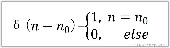
1.单位冲激序列函数
1.2 函数:
1.3 实现代码:
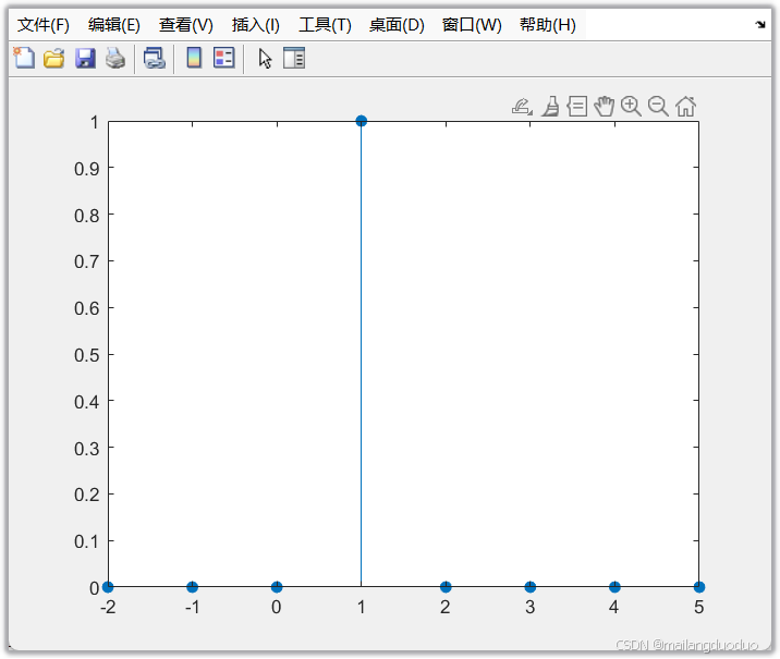
function [x,n] = impseq(n0,n1,n2)% Generates x(n) = delta(n-n0); n1 <= n,n0 <= n2% ----------------------------------------------% [x,n] = impseq(n0,n1,n2)%if ((n0 < n1) || (n0 > n2) || (n1 > n2))error('arguments must satisfy n1 <= n0 <= n2')endn = n1:n2;%x = [zeros(1,(n0-n1)), 1, zeros(1,(n2-n0))];x = (n-n0) == 0;1.3 调用方式
[x,n]=impseq(1,-2,5);
% n=[-2,-1,0,1,2,3,4,5]
% x=    1x8 logical
stem(n,x,"filled")
1.4 调用结果
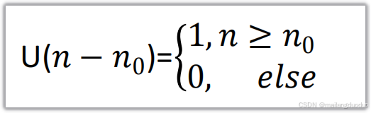
2.单位阶跃序列函数
2.1 函数
2.2实现代码
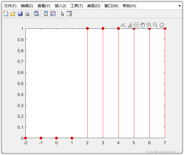
function [x,n] = stepseq(n0,n1,n2)% Generates x(n) = u(n-n0); n1 <= n,n0 <= n2% ------------------------------------------% [x,n] = stepseq(n0,n1,n2)%if ((n0 < n1) || (n0 > n2) || (n1 > n2))error('arguments must satisfy n1 <= n0 <= n2')endn = n1:n2;%x = [zeros(1,(n0-n1)), ones(1,(n2-n0+1))];x = (n-n0) >= 0;2.3调用方式
[x,n]=stepseq(2,-2,7);
% n=[-2,-1,0,1,2,3,4,5,6,7]
% x=1x10 logical
stem(n,x,"filled","r")
2.4调用结果
3.矩形序列
3.1函数
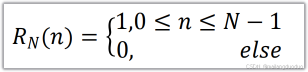
3.2 实现代码
function [x,n]=rectseq(n1,n2,N)
% 个人编写可能有误if n1>=0||n2<n1||n2<N||N<=0error("输入的格式错误");endn=n1:n2;% x=[zeros(1,0-n1),ones(1,N),zeros(1,n2-N+1)];x=bitand(n>=0,n<N);
end
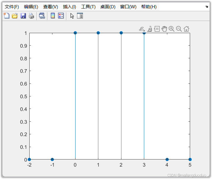
3.3调用方式
[x,n]=rectseq(-2,5,4);
% n=[-2,-1,0,1,2,3,4,5]
% x=1x8 logical
stem(n,x,"filled")
3.4 调用结果
4.实指数序列
4.1函数
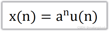
4.2实现代码
function [x,n]=realexpseq(n1,n2,a)
% 个人编写
if n1>n2error("n1应该小于n2");
endn=n1:n2;an=a.^n;x=an.*stepseq(0,n1,n2);
end
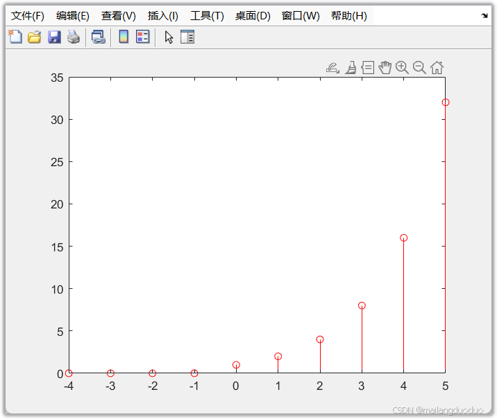
4.3调用方式
[x,n]=realexpseq(-4,5,2);
% n=[-4,-3,-2,-1,0,1,2,3,4,5]
% x=[0,0,0,0,1,2,4,8,16,32]
stem(n,x,"r")
4.4调用结果
5.正弦型序列
5.1函数
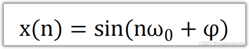
5.2实现代码
function [x,n]=sinseq(n1,n2,w,w0)
%该函数表示sin(w*n+w0)
if n1>n2error("n1应该小于n2");
end
n=n1:n2;
x=sin(w*n+w0);
end
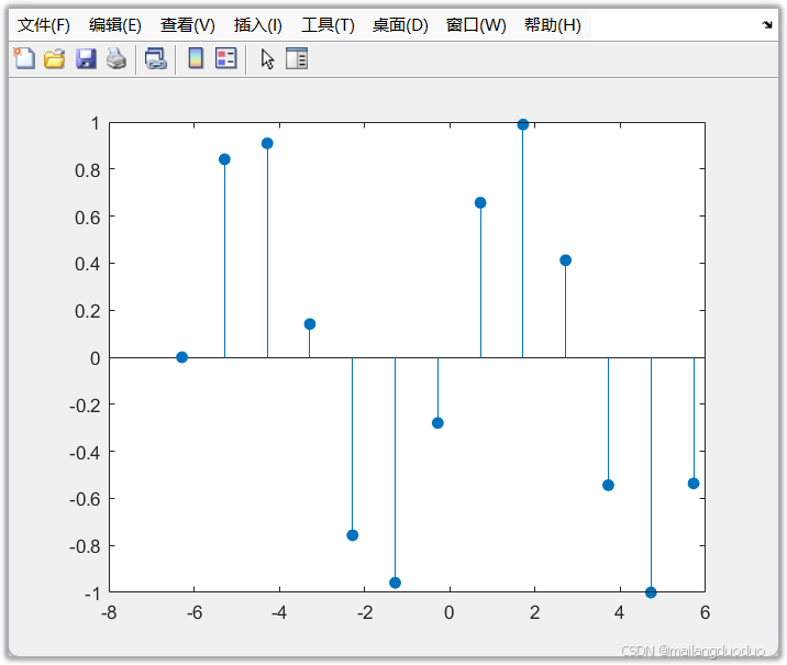
5.3调用方式
[x,n]=sinseq(-pi*2,2*pi,1,0);
% n=1x13 double
% x=1x13 double
stem(n,x,'filled')
5.4调用结果
6.复指数序列
6.1函数
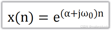
6.2实现代码
function [x,n]=comexpseq(n1,n2,a,w0)
n=n1:n2;
x=exp((a+1i*w0).*n);
end
6.3调用方式
[x,n]=comexpseq(-2,5,2,1);
subplot(2,1,1);
stem(n,real(x),"filled")
xlabel("n");
ylabel("实部")
subplot(2,1,2);
stem(n,imag(x),"filled")
xlabel("n")
ylabel("虚部")
6.4调用结果

备注
以上函数部分是自己写的,部分是以封装好的,可能有些的不足的地方,欢迎批评指正
7.序列的简单运算
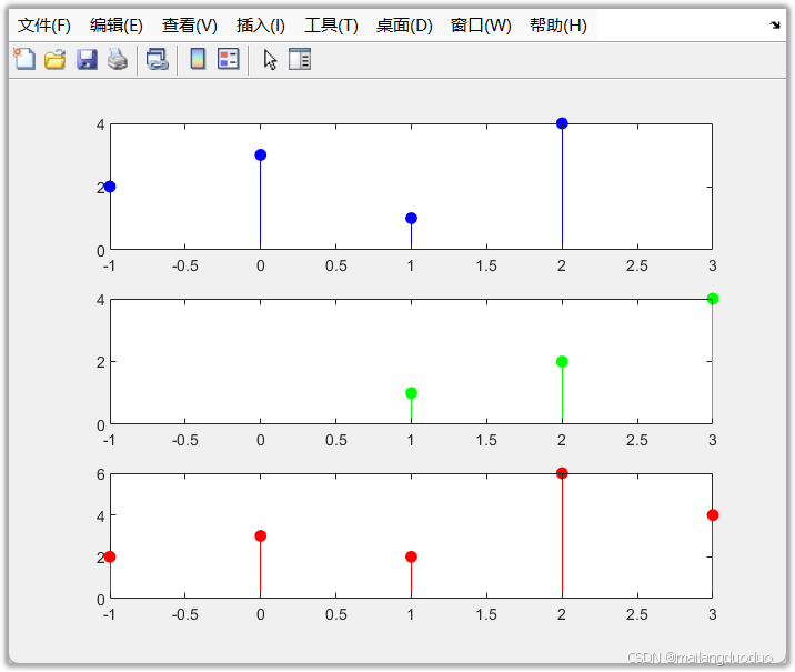
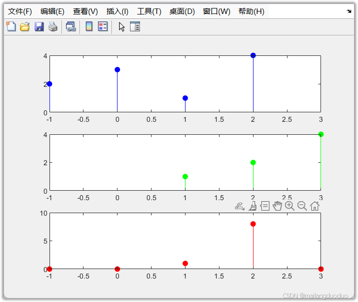
7.1序列相加
将两个序列对应位置直接相加即可
7.1.1 代码实现
function [y,n]=seqadd(x1,x2,n1,n2)n=min([n1,n2]):max([n1,n2]);% 将相加的序列扩展至相同长度y1=zeros(1,length(n));y2=y1;y1((n>=min(n1))&(n<=max(n1))==1)=x1;y2((n>=min(n2))&(n<=max(n2))==1)=x2;y=y1+y2;
end
7.1.2 调用测试
x1=[2 3 1 4];
n1=-1:2;
x2=[1 2 4];
n2=1:3;
subplot(3,1,1);
stem(n1,x1,"filled",'b')
xlim([min([n1,n2]) max([n1,n2])])
subplot(3,1,2)
stem(n2,x2,'filled',"g");
xlim([min([n1,n2]) max([n1,n2])])
[y,n]=seqadd(x1,x2,n1,n2);
subplot(3,1,3)
stem(n,y,"filled","r");
xlim([min([n1,n2]) max([n1,n2])])
7.1.3 调用结果
7.2序列相乘
将两个序列对应位置直接相乘即可
7.2.1 代码实现
function [y,n]=seqmul(x1,x2,n1,n2)
n=min([n1,n2]):max([n1,n2]);
y1=zeros(1,length(n));
y2=y1;
y1((n>=min(n1)&n<=max(n1))==1)=x1;
y2((n>=min(n2)&n<=max(n2))==1)=x2;
y=y1.*y2;
end
7.2.2 调用测试
x1=[2 3 1 4];
n1=-1:2;
x2=[1 2 4];
n2=1:3;
subplot(3,1,1);
stem(n1,x1,"filled",'b')
xlim([min([n1,n2]) max([n1,n2])])
subplot(3,1,2)
stem(n2,x2,'filled',"g");
xlim([min([n1,n2]) max([n1,n2])])
[y,n]=seqmul(x1,x2,n1,n2);
subplot(3,1,3)
stem(n,y,"filled","r");
xlim([min([n1,n2]) max([n1,n2])])
7.2.3 调用结果
7.3序列移位
将序列左移或者右移
7.3.1 代码实现
function [y,n]=seqshift(x,n,m)
% 将序列向左移m位
% y=x(n-m)
n=n-m;
y=x;
end
7.3.2 调用测试
x=[2 4 3 5];
n=1:4;
subplot(2,1,1)
stem(n,x,'filled','g')
xlim([-5,5])
[y,n]=seqshift(x,n,3);
subplot(2,1,2);
stem(n,y,"filled",'r');
xlim([-5,5])
7.3.3 调用结果

7.4 序列翻褶
将序列沿着原点翻褶
7.4.1 代码实现
function [y,n]=seqfold(x,n)
n=-max(n):-min(n);
y=zeros(1,length(x));
for i=1:length(x)y(length(n)-i+1)=x(i);
end
7.4.2 调用测试
x=[4 2 5 3];
n=-1:2;
subplot(2,1,1);
stem(n,x,"filled",'g');
xlim([-4 4])
[y,n]=seqfold(x,n);
subplot(2,1,2);
stem(n,y,'filled','r');
xlim([-4 4])
7.4.3 调用结果

结语
上述函数虽然在Signal Processing Toolbox中都有提供,后续只要会使用即可,本篇博客为了帮助初学者更好的理解各种序列和运算实现的底层过程,为后续学习基于matlab仿真的数字信号处理打下良好的基础。上述代码可能有部分编写不足之处,欢迎批评指出!