政府网站集约化建设 总结郑州做网站推广
ch3中的所有代码,除了在kdevelop中运行,还可以在VScode中运行。下面将简要演示配置过程,代码不再做解答,详细内容在下面的文章中。(这一节中的pangolin由于安装过程中会出现很多问题,且后续内容用不到该平台,所以暂时不进行安装)
视觉SLAM ch3—三维空间的刚体运动![]() https://blog.csdn.net/Johaden/article/details/141023487
https://blog.csdn.net/Johaden/article/details/141023487
其次,我之前的文件推荐了一些软件可以下载,在看下面文章之前,需要至少安装VScode以及git等。
git等常用工具以及cmake![]() https://blog.csdn.net/Johaden/article/details/140715733
https://blog.csdn.net/Johaden/article/details/140715733
下载vscode时会遇到很多问题,可以按照下面的博客逐步下载
ubuntu 20.04系统下安装VSCode(配置C/C++开发环境)![]() https://www.cnblogs.com/icmzn/p/16244665.html
https://www.cnblogs.com/icmzn/p/16244665.html
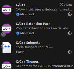
一、基本插件
将命令用不同颜色显示以及tab自动补全。
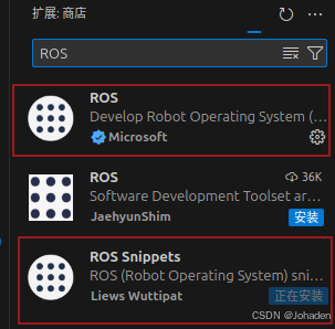
ROS现在暂时用不上,需要的时候再安也行。(建议先不安,拓展安多了容易冲突)
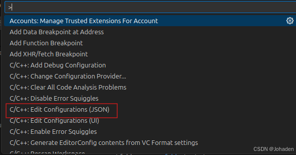
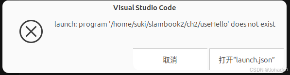
重点:没有Edit Configurations(JSON)怎么办!?
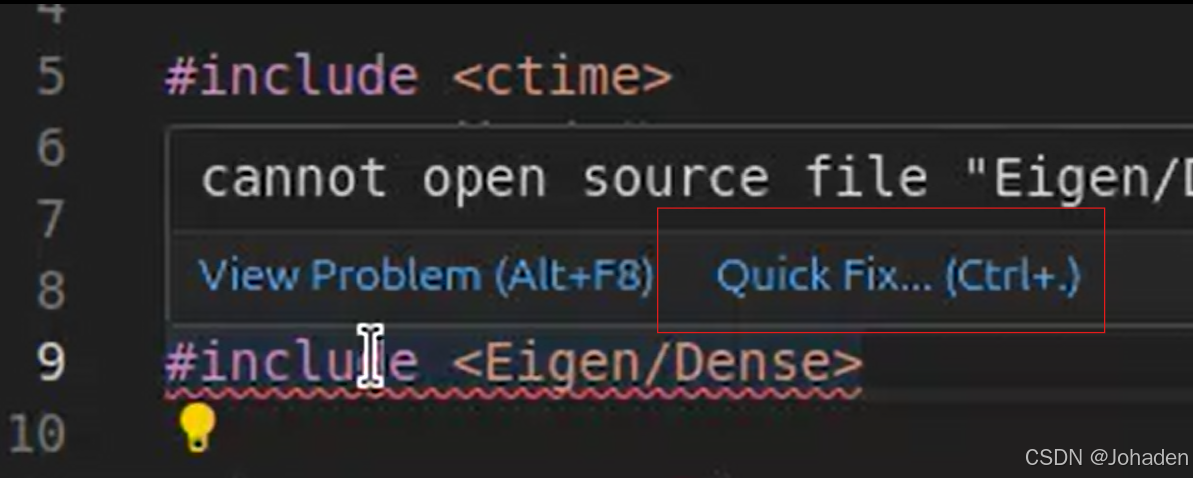
其实这一步是第二部分中需要用到的,但是我在这一步后面卡了两天,现在大家可以现在就自检一下,按ctrl+shift+p后有没有红框内的选项卡,我的刚开始就是没有。
如果你也很不幸,没有这个选项的话(其实C/C++开头的有很多,如果你只有七八个,那肯定就是出问题了),我的建议是不要看网上的别的资源了,因为我看了两天,也实践了两天。无论怎么调整文件、设置都是徒劳的。究其根本就是安装的时候没安好。只能重装了,其实很好装,就是找到这条路的过程是艰辛的。
重装成功之后我也发了一篇博客,链接放在下面了:
在Ubuntu中重装Vscode(没有Edit Configurations(JSON)以及有错误但不标红波浪线怎么办?)![]() https://blog.csdn.net/Johaden/article/details/141193093 重装之后需要重新安拓展
https://blog.csdn.net/Johaden/article/details/141193093 重装之后需要重新安拓展
二、includePath配置
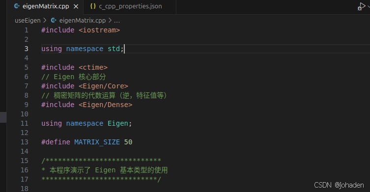
在使用vscode调库的时候,即使我们有头文件,但是总会出现报错,如下图。
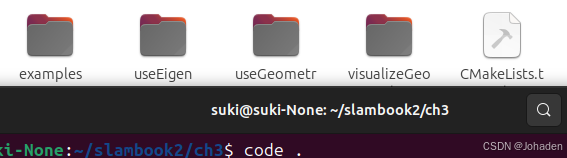
以ch3为例,在ch3中打开终端后输入code .命令后,弹出vscode。
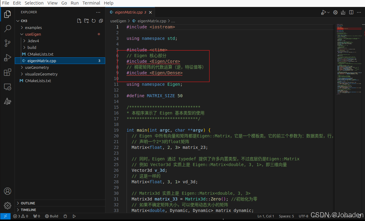
当打开后eigen头文件标红该怎么办?
1.没装过eigen需要自装eigen
sudo apt-get install libeigen3-dev2.方法一:自动修复
方法二:
(1)ctrl+shift+p,选择C++:Edit Configurations(JSON)
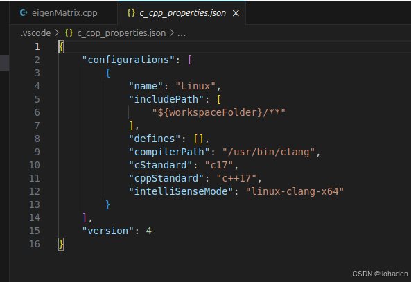
(2)添加库所在位置(使用locate命令查询在哪)
初次使用lacate可能需要安装:
sudo apt install mlocate我们发现当输入locate core的时候,输出了很多个答案,我们也不知道哪个是,所以结合使用grep命令(初次需要安装)
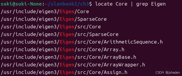
所以我们就知道他们的路径了,也就是/uer/include/engen3/,然后复制下来加在配置文件里。
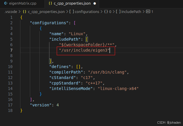
保存后,原来的cpp文件报错消失
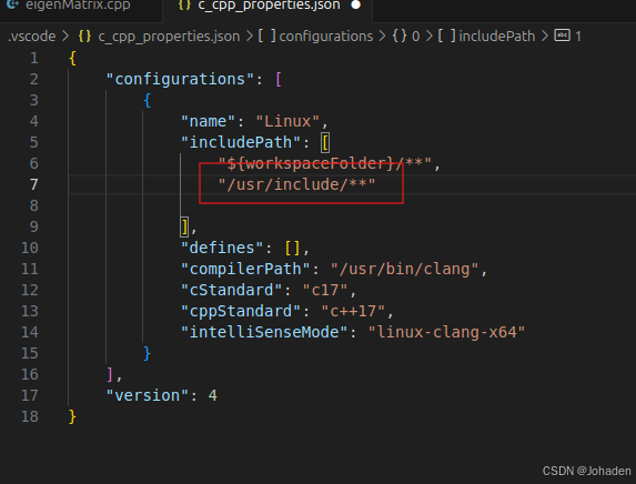
有的时候,/usr/include下面的文件不只是有Eigen,所以如果我们不只是用到了eigen的话,我们只需要使用通配符即可,如下。 (搜索可能比较慢,但是不太容易报错)
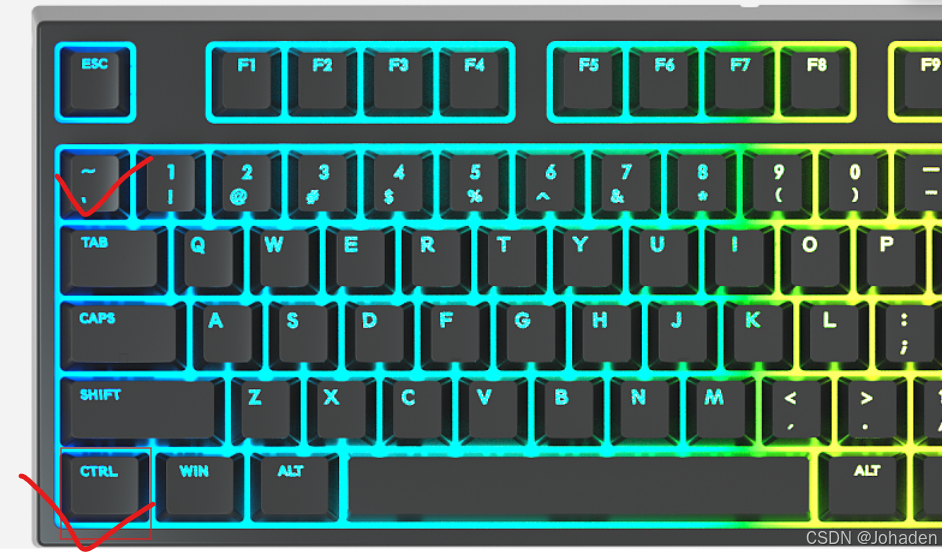
三、嵌入式终端
打开需要按ctrl+·,键位图如下
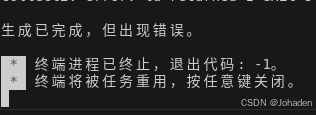
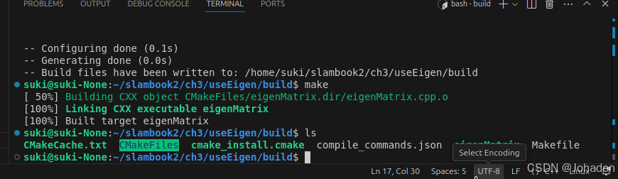
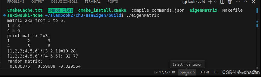
我们可以在里面通过cmake命令生成可执行文件。
(如果你没有build,那就要mkdir build,然后再进去)
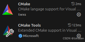
注意:其他功能,比如SSH、Debug都是需要配置的,比较麻烦。未必一定要追求在IDE里运行程序,在写一个大型项目或调试时,一般可以采用直接cout该变量的方式来看该值发生了怎样的变化,调试需要配置的过程非常困难(cmakelist、编译器、setting等)。除非安装一些插件,比如cmake tools,无需配置,直接点击窗口下面的“bug虫”的按钮就行,不做过多介绍。
还有就是删目录的时候,一般都在build下面输入rm -rf *,这个就可以删除全部内容(当然直接在可视化界面删除build文件夹也可以)。但是,用上面命令的时候一定要注意,不要写成rm -rf /*,这会把根目录全删除!!一定要注意!!
四、知识点补充:CMakeLists如何添加Eigen库
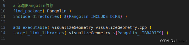
以该处的代码为例,我们不知道它的“包”,也就是动态库在哪里,这时候我们就可以使用find_package(xxx),如果找到了,会返回两个东西,也就是头文件“include_directories(${xxx_INCLUDE_DIRS})”和动态库静态库“target_link_libraries(xxx_LIBRARIES})”
(PS:find_package(xxx)中的xxx必须和xxx.config.cmake中的xxx对应上)
比如之前上一节的代码可以这样写:
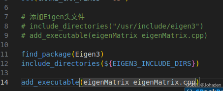
我们怎么知道那个xxx是什么?也就是为什么要写Eigen3?
(1)locate xxx -> include_directories(“路径”)
(2)find_package(xxx):
①REQUIRED:
find_package(xxx REQUIRED) 时,CMake 将尝试定位名为 xxx 的包,并且如果找不到该包,则构建过程将失败,cmake过程会终止,并显示一条错误信息说明缺少所需的包。这确保了在没有正确安装或配置所需依赖项的情况下,不会尝试编译项目,从而避免了潜在的构建失败或运行时错误。
如果不使用 REQUIRED 关键字,即使用 find_package(xxx) ,那么 CMake 会尝试查找包,但如果找不到,它不会终止构建过程,而是简单地继续下去,就像没有找到这个包一样。在这种情况下,你的项目可能需要在运行时动态检查是否存在这些库,或者实现一些替代逻辑来处理缺失的依赖。
②locate xxx | grep 如cmake,就是要找出xxx 相关的 CMake 配置文件。
![]()
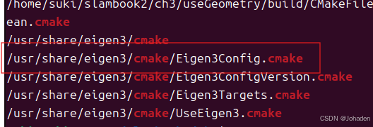
只要找到类似于这个红框的格式,就代表它可以被Eigen找得到。而xxx代表的是Config前面的那个,也就是Eigen3。所以就得到了xxx的格式。
还有,{}里面的是大小写呢?如下,文档中怎么写,这就这么写。
gedit 上面的路径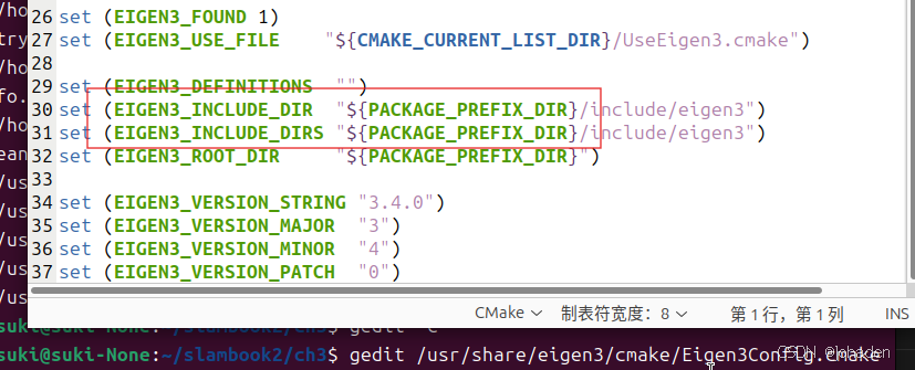
如上图,Eigen文档中写的就是大写,所以我们也要写大写。