网站备案是需要去哪里做登封seo公司
经常看文章时会收获不少实用工具,有的在github上是编译好的,有的则是未编译的项目文件。所以经常会使用Visual Studio编译项目文件成exe可执行程序,以下为编译的流程。
第一步,从github上下载项目文件,举个例子,如工具SharpWifiGrabber
SharpWifiGrabber![]() https://github.com/r3nhat/SharpWifiGrabber
https://github.com/r3nhat/SharpWifiGrabber
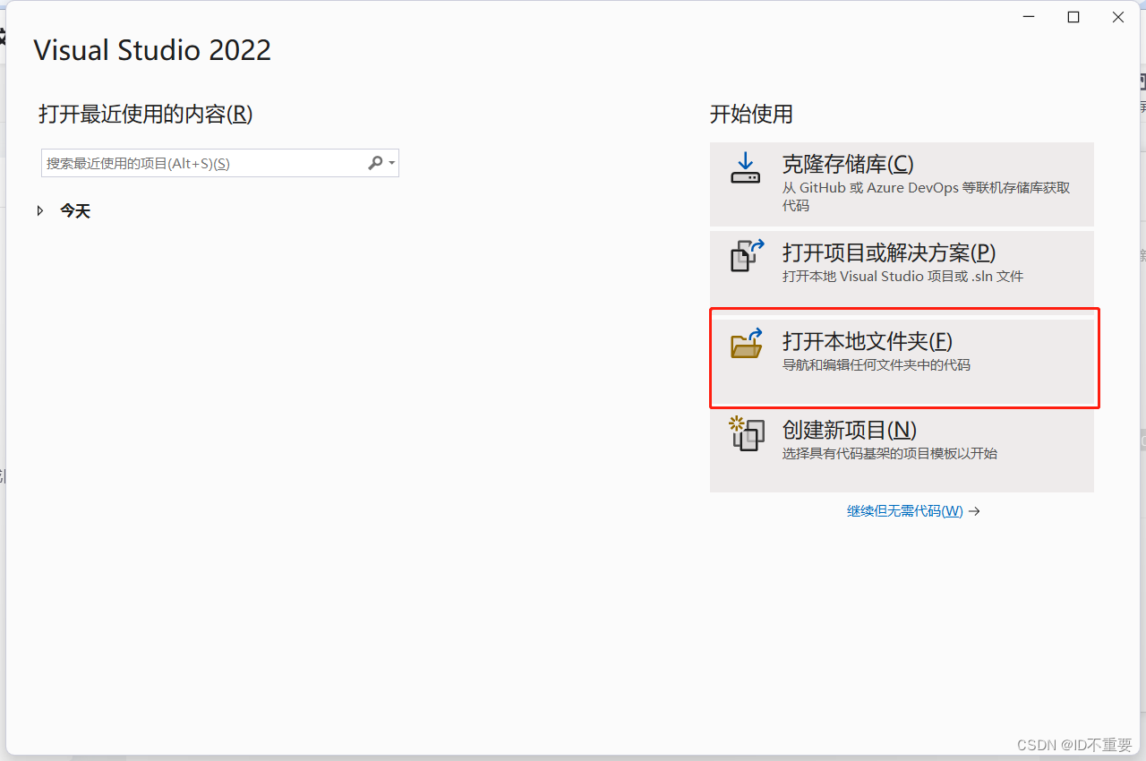
打开Visual Studio
下载解压完成后,打开Visual Studio,选择解压后的本地文件夹
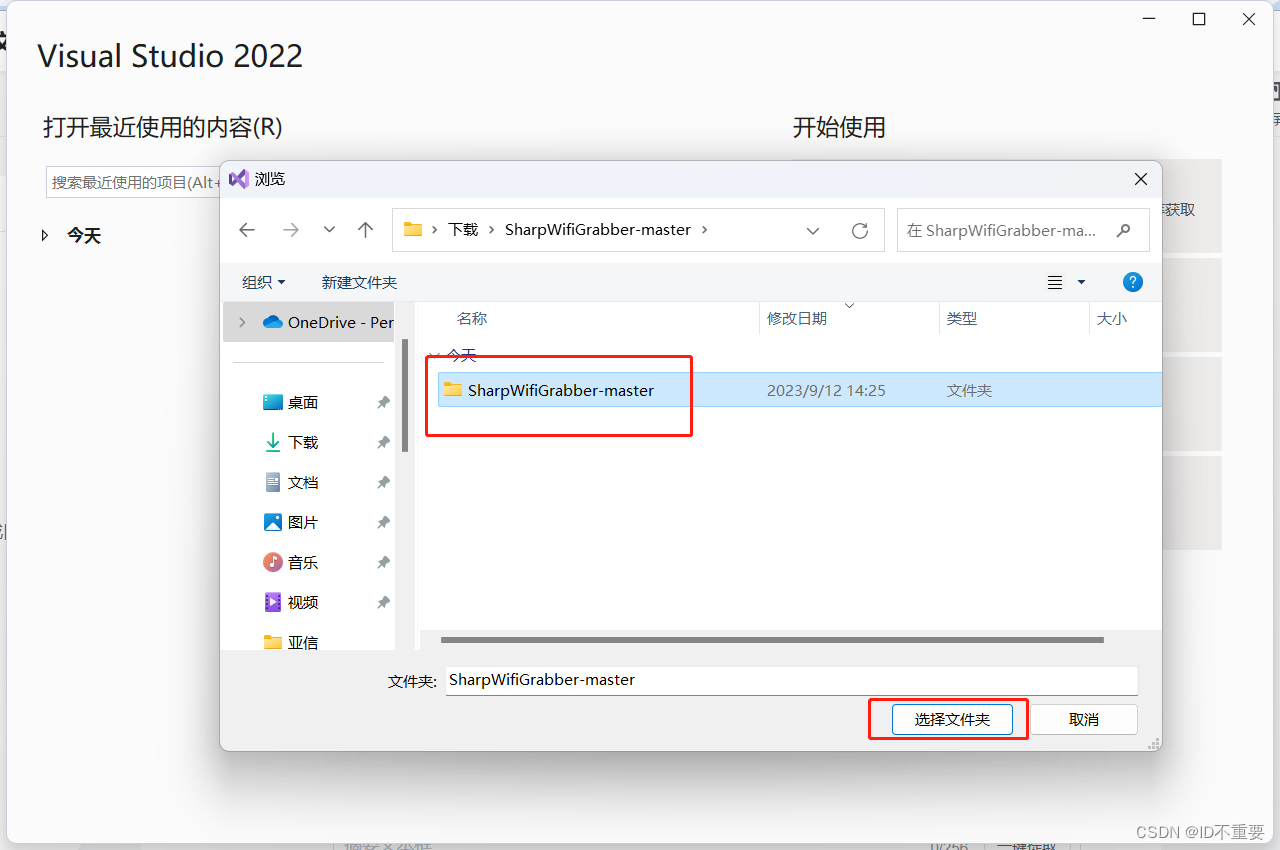
选择项目文件夹
找到文件夹后,选择就行
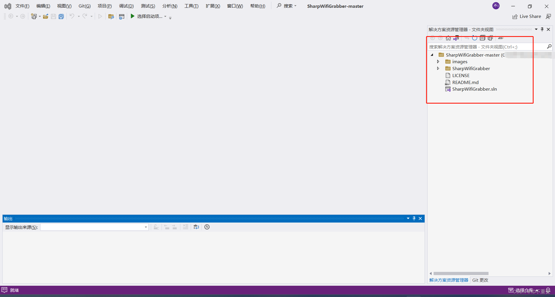
会在右侧出现项目文件
确认依赖环境
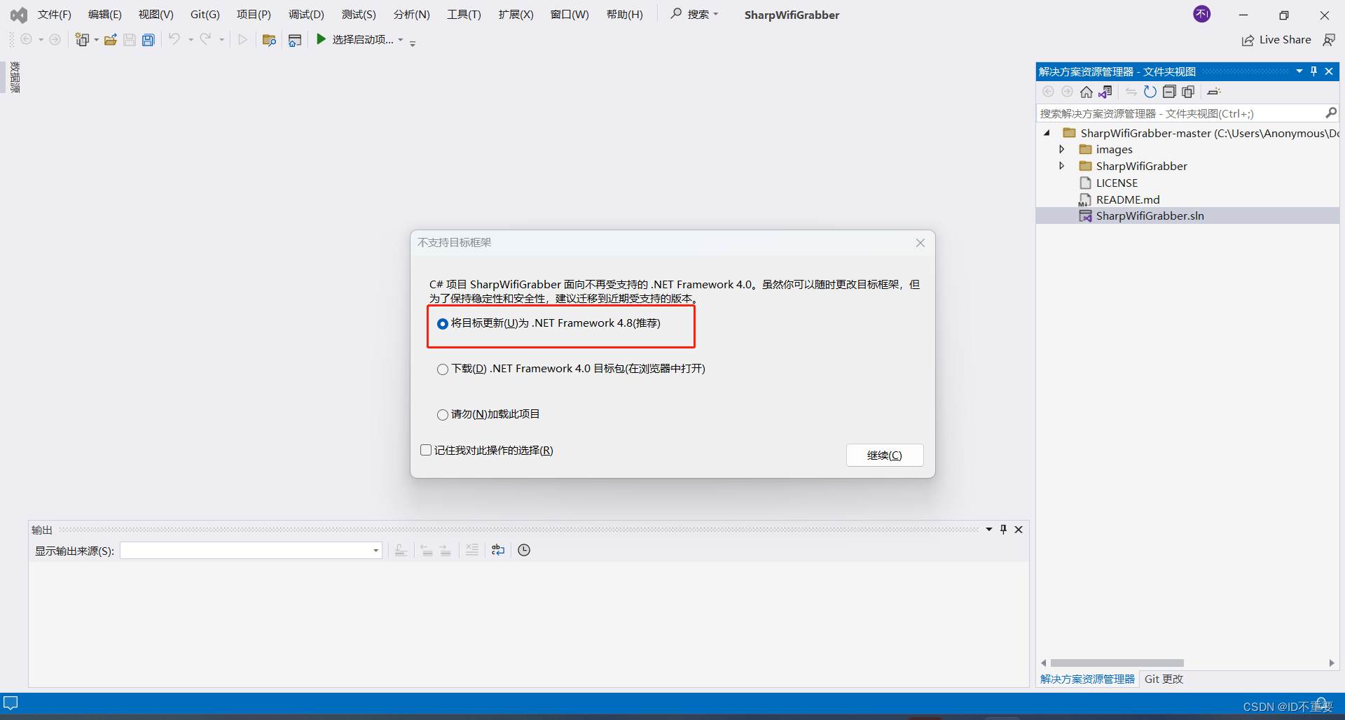
注意,可通过双击sln方案文件来尝试判断依赖环境是否支持,如下图,不支持可选择进行替换,这里选择第一项,替换成.NET4.8
调试程序
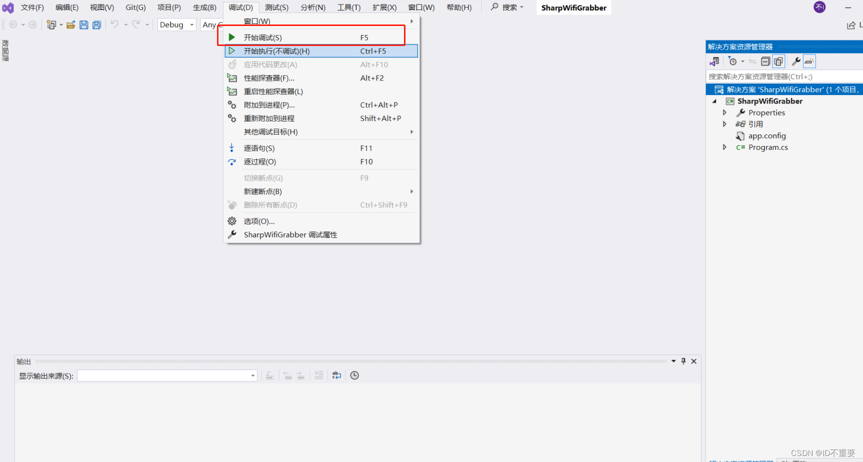
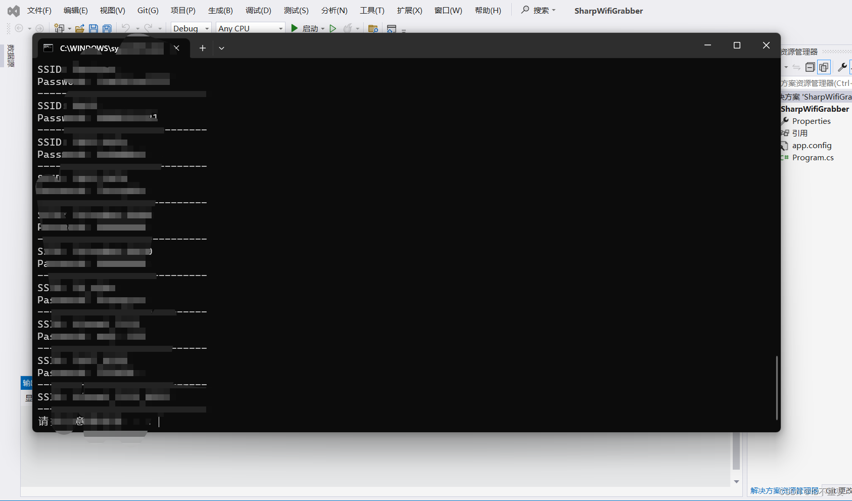
等待片刻更改完成后即可进行调试或开始执行,这里选择开始执行,程序正常执行
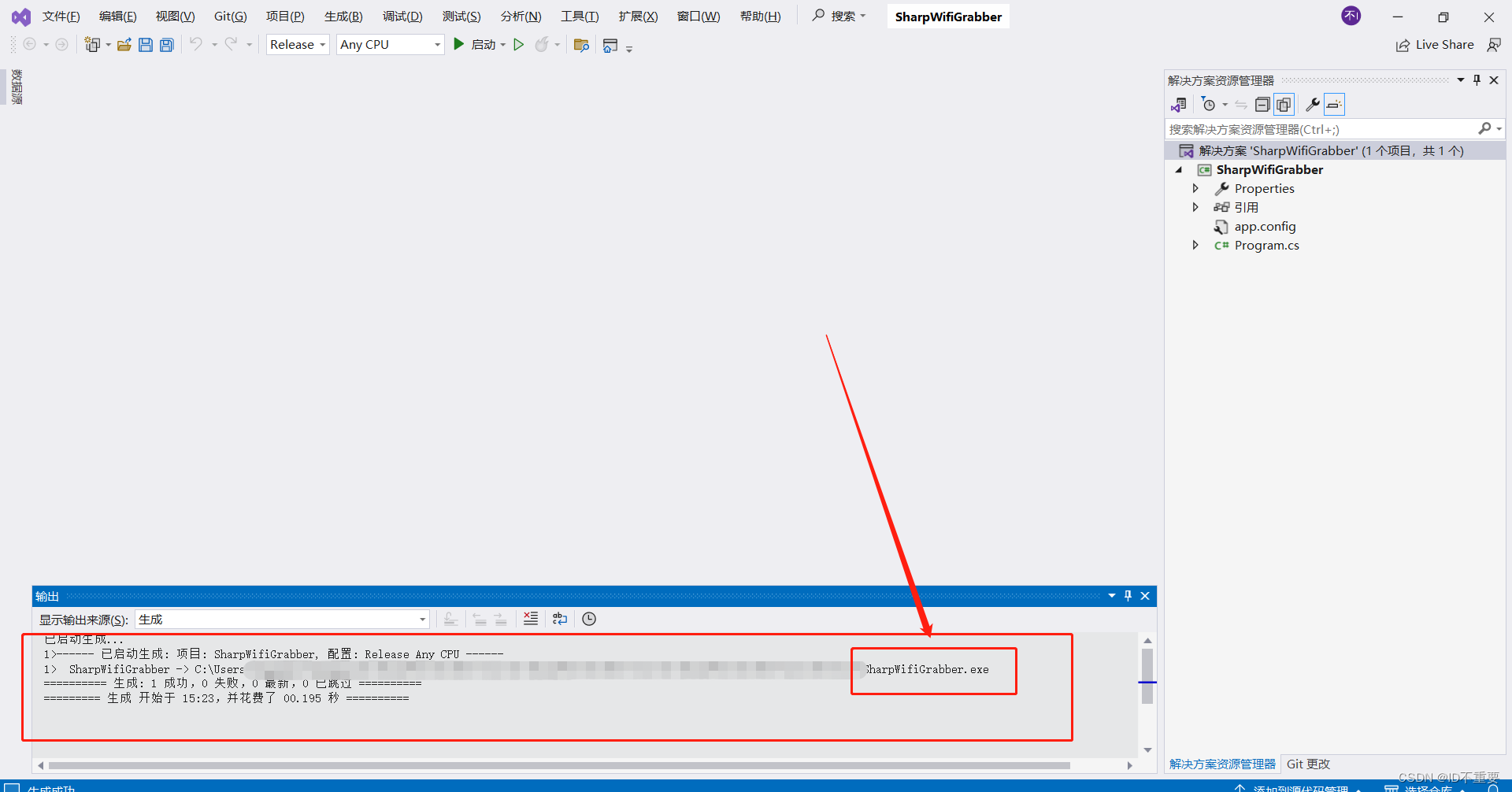
 生成解决方案(可执行程序)
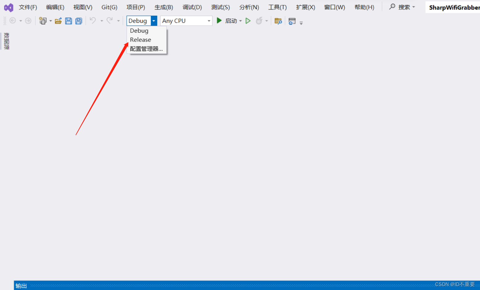
选择Debug或者Release(最终会在项目文件中的/bin目录下生成文件)
点击生成解决方案(可执行程序)
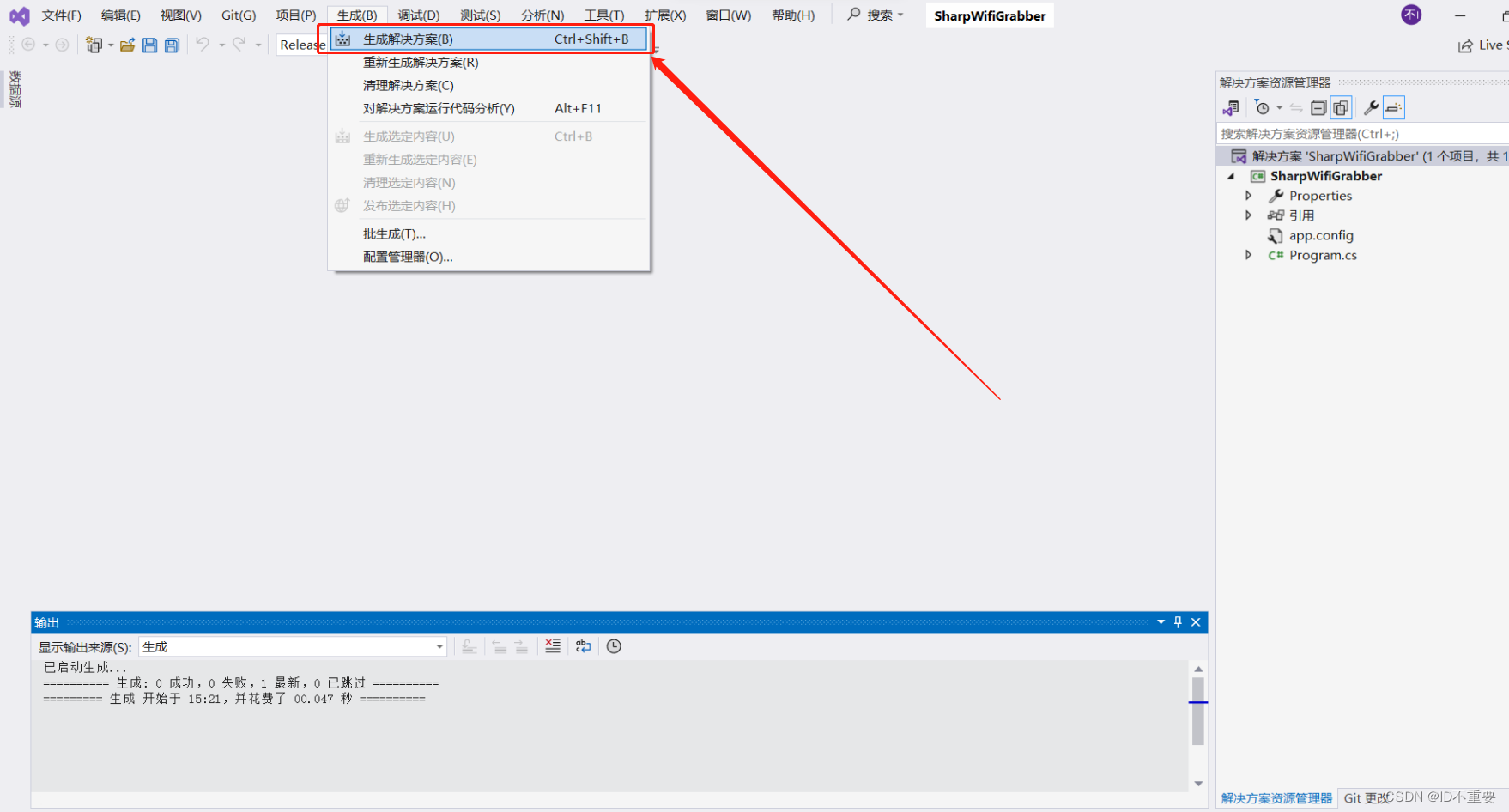
根据路径找到生成的可执行程序