中国关键词网站2345浏览器下载
主要功能是通过红外遥控器模拟控制空调,可以实现根据环境温度制冷和制热,能够通过遥控器设定温度,可以定时开关空调。
1.硬件介绍
硬件是我自己设计的一个通用的51单片机开发平台,可以根据需要自行焊接模块,这是用立创EDA画的一个双层PCB板,所以模块都是插针式,不是表贴的。电路原理图在文末的链接里,PCB图暂时不选择开源。
B站上传的关于这个硬件设计讲解视频链接如下:


1.1 接线定义
| 模块管脚 | 51单片机管脚 |
| LCD1602_RS | P2.0 |
| LCD1602_RW | P2.1 |
| LCD1602_E | P2.2 |
| LCD1602_DB0--DB7 | P0口 |
| 风扇电机正极 | P1.2 |
| 风扇电机负极 | P1.3 |
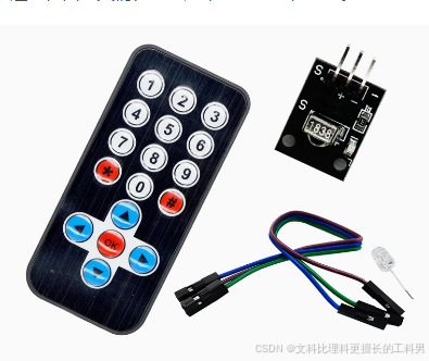
| 红外遥控接收管脚 | P1.6 |
| 制冷继电器 | P1.0 |
| 制热继电器 | P1.5 |
| DS18B20温度传感器 | P2.3 |
2.软件代码
通过分模块化设计,在移植的时候更方便,增减功能的时候只需要修改少量代码即可成功运行。
具体的代码讲解请参考以下B站视频链接:
003-51单片机红外遥控空调_哔哩哔哩_bilibili

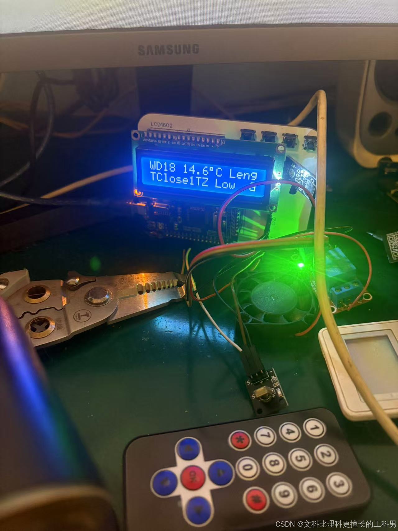
3.实物演示
设定高于温度低于环境温度开始制冷

设定高于温度高于环境温度开始制热
 遥控器调速:Low->Mid->High

定时关闭空调

4.获取源码方式
https://download.csdn.net/download/weixin_41011452/90334072